<strong>Demystifying Hypothesis testing</strong>

Overview

In Management research, one has to understand the principles of Inferential Statistics and Hypothesis testing very well to ensure that the study results are significant, meaning that the results from the study are not merely the result of some random events but are repeatable.

Inferential statistics

In Inferential Statistics we make some inferences about the population characteristics based on a sample. It is often not feasible or it requires enormous resources to commission a study to measure the characteristics of the entire target population and therefore we study the characteristics of a smaller sample ( say > 30 ) to get some sense of a larger population – say the average height of an Indian male, average weight and so on so forth.

So long as the sample size is reasonably large ( say > 30 ) and the sample has been drawn randomly, the sample provides a good insight into the population parameters.

What are the building blocks to carry out the hypothesis testing?

Basic understanding of the concepts of Probability
Probability distribution ( in this paper, we will focus on Normal distribution)
Standard Normal Distribution ( z-distribution) and t-distribution tables
Test statistic ( z value, t value, p value)
Formulation of Null Hypothesis and Alternate Hypothesis

Probability

Most events are probabilistic in nature. When you throw a two-sided, unbiased coin, what is the probability that it will be a Head. It is 1/2 or more generally, Probability (Head) = Number of favorable outcomes / ( total number of possible outcomes) = ½

Unlike the coin tossing example above, most random variables do not have a finite number of outcomes and are continuous in nature. And most random
variables, tend to follow normal distribution. The height of a human being can be assumed to follow a normal distribution. The average height of an Indian male may be around 5 ft and finding someone with a height of 7 ft has a much smaller probability. So, we can safely say that the height is distributed evenly around the mean.

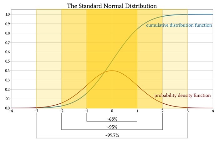
In the figure above, the probability density function follows a normal curve.

In a normal probability distribution function and for that
matter in any probability distribution function (pdf), the values of the random
variable are plotted on the x-axis and the probability density are plotted on the y-axis. Please remember that in a continuous pdf, a point
probability cannot be computed. And the values are clustered around ±1σ ( 68%),
±2σ (95%) , ±3σ (99.7%). This is an important attribute of normal curve which
will come in handy when we do hypothesis testing.

We use normal distribution to measure the probability or the
likelihood of an event happening. The probability of finding someone with a
height of 8 feet or more, let us say, is extremely low and it is measured using
the area of the curve bounded by 8 feet to infinity. The area of the curve
under the tail in the normal curve is very, very low as we move farther and
farther away and hence the probability of an event as we move away from the
mean is quite low. As we have said earlier, the area under ±3-σ is 99.7% and
therefore the area under the tail is only 0.3%. And when the probability of an
event is so low, we can reject the likelihood of that event occurring and that
is the basis for hypothesis testing.

Some Notes on Normal Distribution

The normal distribution approximates many of the natural
phenomena very well and therefore it lends itself nicely for the study of wide
variety of problems.

The random variable under study has to be a continuous
variable.

We will be using a Standard Normal distributions for
Hypothesis testing – a standard normal distribution is nothing but a normal
distribution with a mean of Zero and Variance ( standard deviation ) of one (
1) .

In order to apply standard normal distributions, one must
know the population standard deviation and the sample size must be large say more than 30. In most instances, we do not know the population standard deviation and our sample size may be lesser than 30. In such instances, t-distribution is right model to apply but we will look at a simple case involving z-distribution ( Standard Normal Distribution ) before we segue into t-distribution.

How do we apply Normal Distribution for Hypothesis Testing?

Let us say that you wish to know if the mean obtained from a
random sample of n observations belongs to a population or not with a 95% Level of Significance (LOS). LOS of 95% significance implies that we want to reject the sample as not having come from the population only when the probability is less than 5% – the distance of the sample mean from the mean of the z-curve, measured in terms of the number of standard deviations is more than ±2σ (please recall that ±2σ covers 95% of the area under the normal distribution).

The principal of a private school claims that the IQ of the students who study in his school is way above the average. The average IQ of students in class 12 in the population is 100. And a random sample of 70 students of the concerned private school shows a mean IQ of 120. Does the claim of the school principal agree with the results? Assume that the population standard deviation to be 10.

In order to carry out this test, we first have to state the Null Hypothesis and an Alternate Hypothesis.

In Null Hypothesis, we say that the sample mean is not
different from the population mean and any difference is due to chance.

The Alternate Hypothesis is just the opposite of Null
Hypothesis. When the sample contains sufficient evidence, you reject the Null Hypothesis and conclude that the result is statistically significant and it is not due to chance.

Let’s revisit the principal’s claim that the IQ of students
in his private school is higher than the average. The average IQ in the
population is 100, and a sample of 70 students from this school has an average IQ of 120. Assume that the population standard deviation is known to be 10.

Step 1: Formulate Hypotheses

– Null Hypothesis (H₀): µ = 100 (no difference)

– Alternate Hypothesis (H₁): µ ≠ 100 (two-tailed test)

Step 2: Compute Test Statistic (z-observed)

We calculate the z-score using the formula:

z = (x̄ – μ) / (σ/ √n)

= (120 – 100) /(10 / √70)

= 20 / 1.195 ≈ 16.73

Step 3: Determine Critical Values

For a two-tailed test at 95% confidence, the z-critical
values are approximately ±1.96.

Step 4: Compare and Conclude

Since z-observed = 16.73 > 1.96, we reject the null hypothesis.

Conclusion: There is strong evidence that the students’ IQs
are significantly different (higher) than the population average.

Student's t-Distribution

When the sample size is small ( less than 30), the

application of z-curve to solve problems does not lead to correct results. For
small sample sizes and where we do not know the population standard deviation (
which is often the case), we must apply t-distribution tables.

As the sample sizes are small, the uncertainty from t-tables are more and hence the t-distribution has more area under the tail area. The t-distribution approaches the normal curve as the sample size approaches 30.

And it may be a better idea to apply t-tables for statistical inference as a default strategy.

The method of solving the problems using the t-distribution pretty much follows the same steps that we have outlined before but the formulas are slightly different.

What is a One Sample t-test?

The One-Sample T-Test is a statistical technique used to
determine whether the mean of a sample is significantly different from a known
or hypothesized population mean (μ). This test is particularly useful when:

– The sample size is small (typically n < 30)

– The population standard deviation is unknown

It helps researchers assess whether the observed sample data
could plausibly have come from a population with a specific mean.

Step-by-Step Procedure

Step 1: Formulate the Hypotheses

• Null Hypothesis (H₀): μ = μ₀ (The population mean is equal
to the claimed value)

• Alternative Hypothesis (H₁): μ ≠ μ₀ (The population mean
is not equal to the claimed value — two-tailed test)

Step 2: Calculate the Test Statistic

We use the formula:

t = (x̄ – μ₀) / (s / √n)

Where:

– x̄ = sample mean

– μ₀ = hypothesized population mean

– s = sample standard deviation

– n = sample size

This formula computes how many standard errors the sample
mean is away from the hypothesized population mean.

Step 3: Determine the Critical T-Value

Use the T-distribution table with:

– Degrees of Freedom (df) = n – 1

– Significance level (α = 0.05) for 95% confidence

– For a two-tailed test, divide α by 2 (i.e., 0.025 in each tail)

Step 4: Make a Decision

• If |t_obs| > t_critical, reject H₀

• If |t_obs| ≤ t_critical, do not reject H₀

Alternatively, compute the p-value. If the p-value is less
than α, reject the null hypothesis.

Example: Testing Glucometer Accuracy

Problem:

A manufacturer claims their glucometers measure blood glucose levels with an accuracy of ±10%. To test this claim, a sample of 12 glucometers is selected, and their deviations from the standard value are measured:

Data:

x = [11, 12, 15, 10, 9, 8, 11.5, 12.5, 13, 15, 17, 10.5]

We want to test if the mean deviation is significantly different from the claimed value of 10%.

Step 1: Hypotheses

• H₀: μ = 10

• H₁: μ ≠ 10

Step 2: Compute the Test Statistic

• Sample size (n) = 12

• Sample mean (x̄) = 12.042

• Sample standard deviation (s) = 2.64

• Standard error (SE) = s / √n = 2.64 / √12 ≈ 0.762

t = (12.042 – 10) / 0.762 ≈ 2.679

Step 3: Determine Critical Value

• Degrees of freedom = 11

• α = 0.05 (two-tailed → 0.025 in each tail)

• From t-distribution table: t-critical = ±2.201

Step 4: Decision

• t-observed = 2.679 > t-critical = 2.201

• Therefore, we reject the null hypothesis.

Conclusion

There is sufficient statistical evidence at the 5% level to conclude that the average deviation is significantly different from 10%. The data does not support the manufacturer’s claim about the glucometer’s accuracy.

Hope you find this post useful. If you have any doubts or seek any clarifications, feel free to drop an email – madan.athimoolam@execedonline.co.in

For comments and feedback, write to Madan Mohan Raj, athimoolam.madan@gmail.com, Partner, Centre for Executive Learning. https://execedonline.co.in/